Compressive Sensing Under Matrix Uncertainties and Calibration

In light of the calibration problematic mentioned earlier, this is very timely, here is: Compressive Sensing under Matrix Uncertainties: An Approximate Message Passing Approach by Jason T. Parker, Volkan Cevher, Philip Schniter. The abstract reads:

In this work, we consider a general form of noisy compressive sensing (CS) when there is uncertainty in the measurement matrix as well as in the measurements. Matrix uncertainty is motivated by practical cases in which there are imperfections or unknown calibration parameters in the signal acquisition hardware. While previous work has focused on analyzing and extending classical CS algorithms like the LASSO and Dantzig selector for this problem setting, we propose a new algorithm whose goal is either minimization of mean-squared error or maximization of posterior probability in the presence of these uncertainties. In particular, we extend the Approximate Message Passing (AMP) approach originally proposed by Donoho, Maleki, and Montanari, and recently generalized by Rangan, to the case of probabilistic uncertainties in the elements of the measurement matrix. Empirically, we show that our approach performs near oracle bounds. We then show that our matrix-uncertain AMP can be applied in an alternating fashion to learn both the unknown measurement matrix and signal vector. We also present a simple analysis showing that, for suitably large systems, it suffices to treat uniform matrix uncertainty as additive white Gaussian noise.

GampMatlab is available here, Jason let me know in particular that:

I have added an example of using MU-GAMP to the SourceForge repository. You can find the example in the downloaded zip file here: trunk/code/examples/sparseEstim/muGampExample.m

Also, since I personally cannot run the code because my version of matlab does not do Object oriented scripts, Phil sent me  the following:

....I am attaching a much simplified implementation of MU-GAMP that i wrote for Danny Bickson (who then coded it in his GraphLab and discussed it on his blog http://bickson.blogspot.com/2011/11/gamp-generalized-approximate-message.html).
in this simplified implementation, it is assumed that the signal is bernoulli-gaussian with known statistics, and there is no stepsize-control. it does allow vector- or matrix-valued signals, however.hopefully you will find it useful.
thanks,
phil

Here is the code:

%

 this m-file uses GAMP to estimate the matrix X (of dimension NxT) from the noisy matrix observation Y=A*X+W of dimension MxT. here, A has independent Gaussian entries with matrix mean and variance (A_mean,A_var), W has iid Gaussian entries with scalar mean and variance (0,psi), and X has iid Bernoulli-Gaussian entries with scalar activity rate "lam" and with non-zero elements having scalar mean and variance (theta,phi).

% declare signal parameters
N = 1000; % # weights [dflt=1000]
M = 400; % # observations [dflt=400]
T = 10; % # dimensions per observation [dflt=10]
lam = 0.01*ones(N,T); % BG: prior probability of a non-zero weight [dflt=0.01]
theta = 0*ones(N,T); % BG: prior mean of non-zero weights [dflt=0]
phi = 1*ones(N,T); % BG: prior variance of non-zero weights [dflt=1]
SNRdB = 15; % SNR in dB [dflt=15]
% declare algorithmic parameters
iterMax = 50; % maximum number of AMP iterations [dflt=20]
% generate true Bernoulli-Gaussian signal (i.e., "weights")
B_true = (rand(N,T)>1-lam); % sparsity pattern
X_true = B_true.*(theta+sqrt(phi).*randn(N,T));% sparse weights
% generate measurement (i.e., "feature") matrix
A_mean = randn(M,N)/sqrt(M); % element-wise mean
A_mean2 = A_mean.^2;
A_var = abs(A_mean).^2; % element-wise variance
A_true = A_mean + sqrt(A_var).*randn(M,N); % realization
% generate noisy observations
psi = norm(A_true*X_true,'fro')^2/(M*T)*10^(-SNRdB/10); % additive noise variance
Y = A_true*X_true + sqrt(psi).*randn(M,T); % AWGN-corrupted observation
% initialize GAMP
X_mean = lam.*theta; % initialize posterior means
X_var = lam.*phi; % initialize posterior variances
S_mean = zeros(M,T); % initialized scaled filtered gradient
NMSEdB_ = NaN*ones(1,iterMax); % for debugging: initialize NMSE-versus-iteration
% iterate GAMP
for iter=1:iterMax,
% computations at observation nodes
Z_var = A_mean2*X_var;
Z_mean = A_mean*X_mean;
P_var = Z_var + A_var*(X_var + X_mean.^2);
P_mean = Z_mean - Z_var.*S_mean;
S_var = 1./(P_var+psi);
S_mean = S_var.*(Y-P_mean);
R_var = 1./(A_mean2'*S_var + eps);
R_mean = X_mean + R_var.*(A_mean'*S_mean);
% computations at variable nodes
gam = (R_var.*theta + phi.*R_mean)./(R_var+phi);
nu = phi.*R_var./(R_var+phi);
pi = 1./(1+(1-lam)./lam .*sqrt((R_var+phi)./R_var) .* exp( ...
-(R_mean.^2)./(2*R_var) + ((R_mean-theta).^2)./(2*(phi+R_var)) ));
X_mean = pi.*gam;
X_var = pi.*(nu+gam.^2) - (pi.*gam).^2;
% for debugging: record normalized mean-squared error
NMSEdB_(iter) = 20*log10(norm(X_true-X_mean,'fro')/norm(X_true,'fro'));
end;% iter
% for debugging: plot posterior means, variances, and NMSE-versus-iteration
subplot(311)
errorbar(X_mean(:,1),sqrt(X_var(:,1)),'.');
hold on; plot(X_true(:,1),'k.'); hold off;
axis([0,size(X_true,1),-1.2*max(abs(X_true(:,1))),1.2*max(abs(X_true(:,1)))])
ylabel('mean')
grid on;
title('GAMP estimates')
subplot(312)
plot(10*log10(X_var(:,1)),'.');
axe=axis; axis([0,N,min(axe(3),-1),0]);
ylabel('variance [dB]');
grid on;
subplot(313)
plot(NMSEdB_,'.-')
ylabel('NMSE [dB]')
grid on;
title(['NMSE=',num2str(NMSEdB_(iter),3),'dB '])
drawnow;

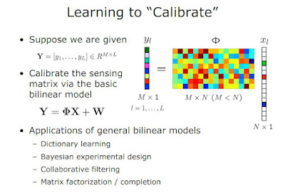
I also was talking to Volkan who pointed me to their similarly relevant paper at SPARS11 (page 68 of the SPARS proceedings) entitled Approximate Message Passing for Bilinear Models. In it, they tackle a specific calibration problem:

"....Example Application: For concreteness, we describe the application of the bilinear model (1) to the compressive system calibration problem. Based on the theoretical premise of compressive sensing, a great deal of research has revolved around the design of sampling systems, such as Analog-to-Information receivers and Xampling. The sampling matrices in these systems are pre-designed with certain desired theoretical properties to guarantee recovery along with the constraints of hardware implementations. However, when implementing the mathematical “sampling” operation—here defined by the matrix Φ—in real hardware, one often introduces what are effectively perturbations on Φ that create an undesired gap between theoretical and practical system performance. As a means of closing this gap, we are interested in jointly learning the true matrix Φ while simultaneously recovering the signal X...."

Attendant presentation slides Approximate Message Passing for Bilinear Models by Volkan Cevher, , Mitra Fatemi, Philip Schniter provide additional insight on this calibration work:

Thanks  Phil, Jason and Volkan. 

Liked this entry ? subscribe to Nuit Blanche's feed, there's more where that came from. You can also subscribe to Nuit Blanche by Email, explore the Big Picture in Compressive Sensing or the Matrix Factorization Jungle and join the conversations on compressive sensing, advanced matrix factorization and calibration issues on Linkedin.