Compressed Sensing: Oil, Curvelets, Missing Data and a Condition on strong CS

There is a new batch of Compressed Sensing articles showing up on the Rice Compressed Sensing site. I am told by Mark Davenport that the site is going to change at some point and will allow for RSS feed. This is good.

Three subjects caught my attention in this batch.

First as usual, the oil people have always been pushing the envelope in terms of devising and using the newest applied mathematics to get things done, so I was not overly surprised to see how curvelets are being used to figure out the layers from seismic measurements. In Non-parametric seismic data recovery with curvelet frames, Felix J. Herrmann and Gilles Hennenfent describe a curvelet-based recovery of seismic signal by a sparsity-promoting inversion technique. This is interesting as this is first time I see an additional matrix added in the inverse problem in order to get rid of data that are necessarily shown by the physics to lead to an ill-posed problem.

With regards to the problem of the missing data problem mentioned earlier, Yin Zhang at Rice asks and begins to answer the question "When is missing data recoverable?" and show how the issue of what you are given in the missing data problem could be construed as a random projections from the real data with the hope that using these measurements you can do a good job of inverting the problem at hand.

Yin is also a co-writer of the Fixed-Point Continuation (FPC) matlab code , An algorithm for large-scale image and data processing applications of l₁-minimization

General l-1 regularized minimization problems of the form

(1)	min ||x||1 + μ f(x),

where f is a convex, but not necessarily strictly convex, function, can be solved with a globally-convergent fixed-point iteration scheme.

Last but not least, Boris S. Kashin and Vladimir N. Temlyakov, A remark on compressed sensing where their equation 1.4 gives a condition I had never seen between the L1 and L2 norm and sparsity number to permit what they call Weak or Strong Compressed Sensing. What we have generally heard before seemed to only be about sparsity number, so I think this is new.

How does the Rice one pixel camera work ?

I have been asked this question several times by colleagues and friends, so I decided to use my talents in Microsoft Paint to try to provide an explanation with some beautifully handcrafted pictures.

The problem to solve is the following: Let's say you have only one sensitive pixel/photodetector/radiation detector/Teraherz detector at your disposal but you need to take a 10 Megapixel image like the one you can get from a Best Buy or an Amazon point-and-shoot cameras how would you go about it ? There are many ways to do this but let us also imagine that you can also put your hands on a DMD chip that is made of 10 million oscillating mirrors (an example include the famous Texas Instrument DMD) like the ones you can find in digital projectors and you can command the action of each and everyone of these tiny (15 micrometer by 15 micrometer) mirrors. In other words, with a proper set-up, every milliseconds, you can decide to shine each of these mirrors on your detector .... or not. There are now two options for obtaining this 10MP image.

First option (the raster mode):

The raster mode is simple. Just shine one mirror at a time onto the detector and let all the other mirros shine elsewhere. Do this once

twice (with another mirror)

thrice (with yet another mirror)
four times (....)
five times (...)
....5 millions times (...)
until you reach the last 10 millionth mirror.

After doing all this, you now have ten million information which put together piece by piece provides you with a 10 MP image. Generally, you then use a small CPU to perform the Discrete Cosine Transform so that eventually you are now the proprietor of a JPEG image (i.e. a compressed version of this 10MP image).

Second option (the Compressive Sensing mode):

You tell the set of mirrors, on that DMD chip, to display a set of random tilings. That way, a random set of mirrors are shining the incoming light unto the detector.

You do this once with an initial random tiling and obtain your first CS measurement

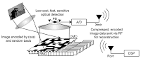
then you do this again with a second random tiling,  in order to obtain your second CS measurement

then you do this again with a third random tiling,  this is your third CS measurement
and so on.

Compressed sensing tells you that with very high probability, you will get the same result as the raster mode (first method) above but with many fewer CS measurements than the 10 million raster mode measurements obtained in the first method. In fact, instead of taking 10 million raster mode measurements, you are likely to need only 20 percent of that in the form of CS measurements, maybe even less.

The reason this second method works stems from the idea that most natural images are sparse in bases ranging from cosines, wavelets to curvelets (this is also why JPEG does a tremendous job in decreasing the size of most images). Functions that represent random tilings of reflective and non reflective mirrors (0s and 1s) are said to be mathematically "incoherent" with these bases thereby allowing an automatic compression at the detector level (here in the second mode, there is no need for compression with JPEG at the very end since the CS measurements are already compressed version of the image). A computational steps is required to obtain a human viewable image from these CS measurements. That step uses these solvers.

What are the pros and cons of the second option compared to the first one ?
Pros:

1. The overall sensor requires very low power because there is no CPU/GPU/FPGA trying to perform the compression stage at the very end (JPEG).
2. The sensor is dedicated to acquiring information. Information processing can be done somewhere else ( think on some other planet)
   
3. Compared to raw images (raster mode output), the information to be transmitted is very much compressed albeit not optimally (compared to JPEG).
4. Instead you can spend all your money designing the very best sensitive pixel you want, it may even act as a spectrometer (looking at many different energy bands), radiation detector and so forth.
5. Last but not least, the amount of light that goes to the detector is about half of the 10 million mirrors, which is quite high compared to the single mirror exposure in the raster mode (first method). In other words, the signal to noise ratio is pretty high (a good thing) in the CS mode as opposed to the raster mode.

Cons:

1. Faint signals could be submerged in the CS measurements. You first need to have a high signal to noise ratio signal to detect small signals.
2. Your sensor has to have a much larger dynamic range than in the raster mode in order for the A/D quantization algorithm to not mess with the CS measurements.
3. The number of CS measurements will be higher than the number of bits required to store the JPEG of the raster mode (about 4 to 5 times higher). Then again (and this is a pro-argument, the transformation from raster mode to JPEG is the power hungry stage of your camera and the reason you always need to recharge it, memory on the other hand is cheap.)

Terry Tao provides a much clearer mathematical explanation albeit with no beautifully hand crafted images such as the ones found here. All information about this single pixel camera system can be found at Rice University.

[ Update 2013: Inview Corporation develops single pixel cameras using the intellectual property from Rice University ]

Tree based pursuit

Make that six codes enabling the reconstruction of a signal using an overcomplete dictionnary. Philippe Jost at EPFL is making available the TREE BASED PURSUIT 2D toolbox. According to his abstract:

Tree-based pursuit efficiently trades off complexity and approximation performance for overcomplete signal expansions. Finding the sparsest representation of a signal using a redundant dictionary is, in general, a NP-Hard problem. Even sub-optimal algorithms such as Matching Pursuit remain highly complex. We propose a structuring strategy that can be applied to any redundant set of functions, and which basically groups similar atoms together. A measure of similarity based on coherence allows for representing a highly redundant sub-dictionary of atoms by a unique element, called molecule. When the clustering is applied recursively on atoms and then on molecules,it naturally leads to the creation of a tree structure. We then present a new pursuit algorithm that uses the structure created by clustering as a decision tree. This tree-based algorithm offers important complexity reduction with respect to Matching Pursuit, as it prunes important parts of the dictionary when traversing the tree. Recent results on incoherent dictionaries are extended to molecules, while the true highly redundant nature of the dictionary stays hidden by the tree structure.

Nothing short of a revolution, part 3 : It does not need to be nonlinear

And then something happened in 1999: Emmanuel Candès and David Donoho noticed that with curvelets, one did not need an adaptive or a nonlinear scheme to converge on images with edges[1]. This is important because as stated before, the only way people were using wavelets and related functions (ridgelets,...) was through a nonlinear scheme, i.e. compute all the wavelet or fourier coefficients first and then do a threshold on them in order keep only the largest ones. While in the wavelet case, i.e. in 1-d, the issue is not really a big deal, it becomes a nightmare when you try to use this type of technique in multidimensional spaces. If you have to compute all the moments of an integral equation and then remove the ones that are too small (because wavelets sparsify certain integral kernel), you have barely made progress over the state of the art like fast multipole methods. So for the first time since the arrival of wavelets, there is hope that there is a linear process by which one can produce a sparse representation of a function or set of data. Ok so now we have a way to get a truely sparse approximation of a function using basis pursuit, we have tons of nice families of functions to do this and we now know that in order to find a sparse representation of a function we don't need a nonlinear scheme, why is this related to compressed sensing ?....

References

[1] Curvelets - a surprisingly effective nonadaptive representation for objects with edges. Curves and Surfaces, L. L. Schumaker et al. (eds), Vanderbilt University Press, Nashville, TN. Compressed Postscript (ps.gz) / (pdf)

Nothing short of a revolution. Part deux: Pursuing a dream

With the wavelet bang came another realization and then something odd happened. In 1994, Donoho and Chen published a paper that summarized the state of the affairs on approximation:

- The realization that now, with wavelets of all kinds being added daily on top of the old approximating polynomials, there are too many functions to be used to decompose a signal and there is no good way in figuring out which one is the best to use. The situation is so bad that you can write an entire dictionnary of different wavelet names.

- Some signals are a composition of various functions and distributions (diracs,...), so it does not make sense to decompose them with respect to only one family of function. If you use only one type of decomposing function, you will not get a sparse decomposition. Take for instance the case of Gibbs phenomenon where one tries to approximate a dirac with a bunch of sines and cosines.

- Most decomposition algorithms are based on a least square approach. In other words, the criterion with which one decides whether a series of approximation has converged in based on a $L_2$ distance or the euclidian distance. The definition of a scalar product is therefore essential but no one knows why some scalar products work better than other. In the end, many formulation of a variety of engineering problems rely on so-called weak formulation such as the finite element method but sometimes, no one knows really why they should be using these methods. Case in point, albeit a non traditional one: Neutron and Radiation Transport. There are many weak formulation of the linear transport equation even though we know that it has distribution as eigenfuctions. Yet neither the scalar product of the weak formulation ($L_2$) nor the one induced by the scalar product of the eigendistribution can constrain any of the solution to be positive (an initial requirement) or have a direct physical meaning.

- If the scalar product is induced by the decomposing family of function, then how can one try to decompose a function simultaneously along different set of functions ?

- The $L_2$ distance criterion never converges toward a local approximation. The approximation will have many coefficients that are very close to each other. There will be no way to apply a blind threshold to these coefficients because each and everyone of them count in the minimization of the criterion.

- The problem that you have always wanted to solve is an $L_0$ problem not an $L_2$. The $L_0$ is the criterion is really about the sparsity of the approximation.

- $L_0$ problem is NP-complete so there is no way you can figure a solution in your lifetime on average.

Donoho and Chen showed that if you were to solve an $L_1$ problem instead of an $L_0$, the solution was likely very close to the $L_1$. Solving an $L_1$ problem is akin to performing linear programming or an optimization. Because of its over reliance on least square approach, the whole engineering field could be shattered as a result. Yet, the method by which one can obtain a solution are significantly time consuming at that time that it was not likely to make a dent in the weak formulation business anytime soon. The lingering thought is still that it will eventually prevail and change our views on how to solve engineering problems in the future. At some point, even Google was using some code word related to the $L_1$ approach to find future employees :-). There needs to be other stepping stones to reach the final climax of this story though.

Nothing short of a revolution. Part I: When a scam can kill you

This story is about the revolution brought about by compressed sensing or compressive sampling. It is a beautiful story as far as I can tell and I will try to parse it in three or four parts. I write it as an outsider and I therefore hope to be forgiven if I missing names.

It all started with the (re)discovery of wavelets by Jean Morlet and the work of people like Alex Grossman. The field was expanded by people like Yves Meyer, Stephane Mallat, Ingrid Daubechies and many others. As pointed out in the text about Jean Morlet, it all started badly:

...Until now, his only reward for years of perseverance and creativity in producing this extraordinary tool was an early retirement from Elf...

Elf was not fearing knowledge or fearing to be more competitive but rather the company had been hit with a scandal that nearly shattered a government and a presidency. The avions renifleurs affair (sniffer planes) made most of the management at ELF very cautious/squeamish about any type of extraordinary scientific announcement. So when Morlet came in and told people about wavelets, they had him retire. While the story is cute, it took a good ten years before wavelets became of interest in the generic engineering literature.

As an engineer myself, the turning point for making these functions useful was when Dave Donoho started to make available a series of routines on the internet so that other researchers could reproduce his own published material (David Donoho wants his research to be reproducible because he thinks that publication is not scholarship but merely an advertisement for it). The Wavelab toolbox was revolutionary because, in effect, since most of these wavelet functions were not analytic (they are mostly defined as a solution to a recurence relation) most engineers had to first build something to get to see a "wavelet" function. And while there were wavelets built from spline functions by Chui, Goswami and Chan these never really took off in the literature. Wavelets are now routinely used in every areas of engineering and have joined Fourier analysis in the series of tools engineers and scientists use in their daily lives. They have changed the face of applied harmonic analysis and change our ways we look at signals such as image, voice, etc. However, the revolution only starts here. The bigger boom came from another area of mathematics...

WITS, a collection of links to choose wavelets and other related functions.

Ths WITS lists a pretty complete collection of links to functions such as wavelets, ridgelets, curvelets, contourlets, bandelets and other beamlets. With the increase in the number of families of functions needed to study higher dimensional spaces (above 1), it is a very good idea. Some of these codes are available in matlab.

Basis Pursuit

Here is a very interesting paper on the use of Basis Pursuit to find a correlation between different parametric models and data from time dependent PET scans. The nice thing that makes it clear is that there is no need for an ad-hoc procedure to make sure that some coefficients are non-negative (non physical.) We have this kind of problem in neutron transport. In that area, ways to deal with this type of problems are called flux fixing.