Ken Clarkson left a new comment on a previous post "OSNAP: Faster numerical linear algebra algorithms ...":
Hi. While Huy and Jelani have sharper results, and cleaner proofs, it's worth mentioning that David and I have sharpened our analysis as well, reducing O(nnz(A)log ) to O(nnz(A)) dependence in that second set of results for us in their table, for regression and low-rank approximation. These improvements result from a more careful analysis in the heavy-coordinate, "perfect hashing", part of our proof; they are in the current version of our paper on arXiv.
My bad, indeed, David states so in the video, the log factor is gone. (slides are also listed in the recent Workshop on "Randomized Numerical Linear Algebra (RandNLA): Theory and Practice"). Thanks Ken !
Again, I hesitate to mention that this is an implementation as the hashing mechanism seems so trivial. The arxiv paper is: Low Rank Approximation and Regression in Input Sparsity Time by Ken Clarkson, David P. Woodruff
(Submitted on 26 Jul 2012 (v1), last revised 31 Oct 2012 (this version, v3))
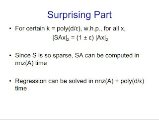
We design a new distribution over $\poly(r \eps^{-1}) \times n$ matrices $S$ so that for any fixed $n \times d$ matrix $A$ of rank $r$, with probability at least 9/10, $\norm{SAx}_2 = (1 \pm \eps)\norm{Ax}_2$ simultaneously for all $x \in \mathbb{R}^d$. Such a matrix $S$ is called a \emph{subspace embedding}. Furthermore, $SA$ can be computed in $\nnz(A) + \poly(d \eps^{-1})$ time, where $\nnz(A)$ is the number of non-zero entries of $A$. This improves over all previous subspace embeddings, which required at least $\Omega(nd \log d)$ time to achieve this property. We call our matrices $S$ \emph{sparse embedding matrices}.Using our sparse embedding matrices, we obtain the fastest known algorithms for $(1+\eps)$-approximation for overconstrained least-squares regression, low-rank approximation, approximating all leverage scores, and $\ell_p$-regression. The leading order term in the time complexity of our algorithms is $O(\nnz(A))$ or $O(\nnz(A)\log n)$.We optimize the low-order $\poly(d/\eps)$ terms in our running times (or for rank-$k$ approximation, the $n*\poly(k/eps)$ term), and show various tradeoffs. For instance, we also use our methods to design new preconditioners that improve the dependence on $\eps$ in least squares regression to $\log 1/\eps$. Finally, we provide preliminary experimental results which suggest that our algorithms are competitive in practice.
and here the video:
Low Rank Approximation and Regression in Input Sparsity Time, David Woodruff


3 comments:
Hi,
My bad, indeed, David states so in the video, the log factor is gone.
Sorry to add more confusion to the mix, but I don't think this is what Ken meant (in particular, the video you link to is from before what Ken is talking about). Their work was always, from the first version, able to get nnz(A) + poly(d/eps) time for regression, without the log n. What Huy and I addressed was: how big is the poly? Originally the CW12 poly was d^5*polylog(d), and they were able to make it d^3*polylog(d) (even replacing d with rank(A)) at a sacrifice: by turning nnz(A) into nnz(A)*log n. I think Ken's point is that they no longer have to make that sacrifice with their Oct. 31st version: their sharpened analysis can make it d^3*polylog(d) while still keeping the log n term away from the nnz(A). (See footnote 2 in our manuscript.)
The point of what we did is that (a) it's nnz(A) + d^3*log d, with only one log d multiplying the d^3 term (this difference used to be d^3*log d vs. d^5*polylog(d), and now is d^3*log d vs. d^3*polylog(d) given the Oct. 31 version that Ken referred to; I think this is what Ken's point was in his comment), and (b) if you're willing to make the sacrifice of multiplying nnz(A) by log n then you can make the additive term be d^{omega+gamma} for arbitrarily small gamma>0 (and again, d can be replaced with rank(A) in this bound), where omega < 2.373 is the exponent of matrix multiplication. There are some other differences also, e.g. our analyses don't need as strong hash functions to go through which has some slight advantages in streaming settings (see the paper).
I guess I should have mentioned that even for (b) above, you actually don't even have to multiply nnz(A) by log n to get d^{omega+gamma}; rather, you have to multiply nnz(A) by a constant depending on 1/gamma. You do multiply it by log n if you want rank(A)^{omega+gamma} time though.
Thank you Jelani ( http://nuit-blanche.blogspot.com/2012/11/a-note-from-jelani-nelson-on-osnap.html )
Post a Comment