Le Gout des Autres - The Taste of Others

Sometimes, I don't write entries on Compressive Sensing. This is one of these occurences. Since mid-December, I have lost about nineteen pounds (8.5 kg) by following some of the results of the self-experimentation of Seth Roberts, a professor at Berkeley (you need to read his fascinating blog here). What did it take to do this ? For me, just one thing: a $4 nose clip that I put on my nose every time I eat. That's it. No exercise. I eat what I usually eat although now in a rather lower amount (not because I am starving myself but because I feel full earlier). At the start of this trial, the weight loss was pretty steep. Since putting a nose clip has some social cost I lose it when I eat out with friends or through the Christmas period. The underlying theory given by Seth is that we are not wired for food developed in the past fifty years (lots of what we eat is highly processed and engineered for one purpose: to be eaten) . By decoupling the food intake with its smell, our brain is less capable in determining whether that intake should be stored or not. Anyway, I can now see abs that I had not seen for the past twenty years. Which brings me to this other 20 year old find: I was going through my stuff and found the first e-mail I ever received from France. It's a response to an e-mail I had sent a friend. Enjoy:

From: Jnet%"OPER@FRCIME51" 19-JAN-1989 17:28:26.35
To: *******@TAMSIGMA
CC:
Subj:

Received: From FRCIME51(OPER) by TAMSIGMA with Jnet id 0037
for *******@TAMSIGMA; Thu, 19 Jan 89 17:28 CST
Date: 19-JAN-1989 12:31:05.51
From: OPER@FRCIME51
To: *******@TAMSIGMA
Subj: RE: ENCORE LUI

Les comptes etudiants n'ont pas acces aux messageries internationales ni meme nationales...
Merci de ne pas encombrer les reseaux.

which translates into:

Students' acounts do not have access to international or even national E-mail...
Thank you for not overloading the network.

It sounds as if I was clogging the tubes or maybe the postmaster did not find my initial E-mail to his taste.

CS: Streaming, One pixel Color Camera, CS and RTE, a request, Multi-Label Prediction via CS, Blind reconstruction,

First off Congrats to Ramesh Raskar for his Sloan Fellowship (he is still looking for some folks to join his group). Second, it looks like the compressive sensing workshop is a success but it looks like the coffee person messed with thee tea pot.

Piotr Indyk has a series of lecture he is giving at Rice this spring on the relationship between streaming and compressive sensing. The lectures are here.

From the Rice Compressive Sensing resource site, here is a new paper:


Compressive Imaging of Color Images by Pradeep Nagesh and Baoxin Li. The abstract reads:

In this paper, we propose a novel compressive imaging framework for color images. We first introduce an imaging architecture based on combining the existing single-pixel Compressive Sensing (CS) camera with a Bayer color filter, thereby enabling acquisition of compressive color measurements. Then we propose a novel CS reconstruction algorithm that employs joint sparsity models in simultaneously recovering the R, G, B channels from the compressive measurements. Experiments simulating the imaging and reconstruction procedures demonstrate the feasibility of the proposed idea and the superior quality in reconstruction.

It looks like the RGB encoding could also be useful for smell encoding as well. When are we going to see a compressive sensing nose ? The bayer pattern reminds me of a previous post on retinal cells.

On Friday, March 13, 2009, Hongkai Zhao will give a talk at Stanford on "A fast solver for radiative transport equation and applications in optical imaging". The Abstract reads:

I will present an efficient forward solver for steady-state or frequency-domain radiative transfer equation (RTE) on 2D and 3D structured and unstructured meshes with vacuum boundary condition or reflection boundary condition. Due to high dimensionality the key issue is to construct an efficient iterative scheme that can deal with various behaviors of the solution in different regimes, such as transport, diffusion, optical thick, and forward peaking . In our algorithm we use a direct angular discretization and upwind type of spatial discretization that preserves properties of both scattering and differential operators of RTE. To solve the large linear system after discretization, we construct an efficient iterative scheme based on Gauss-Seidel and proper angular dependent ordering. With this iterative scheme as the relaxation we implement various multigrid methods in both angular and physical space. Our algorithm can deal with different scattering regimes efficiently. Efficiency and accuracy of our algorithm is demonstrated by comparison with both analytical solutions and Monte Carlo solutions, and various numerical tests in optical imaging. Based on this algorithm, a multi-level imaging algorithm is developed for optical tomorgraphy. If time permits, I will also talk about recent work on compressive sensing (CS) in bioluminescence tomography (BLT) based on RTE. We show that direct use of Green's function of RTE as the basis and standard measurement data for reconstruction will not satisfy the restricted isometry property (RIP). We propose an algorithm to transform the standard setup into a new system that satisfies the RIP. Hence, with compressive sensing method, we produce much improved results over standard reconstruction method.

Three items of interest of mine collide here. The RTE or linear transfer equation or Boltzmann equation, compressive sensing and finally the usefulness of RIP. Again running the risk of repeating myself, which I do quite often:The RIP is a sufficient condition, if it does not work out for your problem then maybe you should look at a low order model of your problem and see how it fits into another sufficient (expected to be stricter) condition namely the one calculated in On verifiable sufficient conditions for sparse signal recovery via L1 minimization by Anatoli Juditsky and Arkadi Nemirovski. An implementation is available at this site:

http://sites.google.com/site/testsensingmatrices/

or in Testing the Nullspace Property using Semidefinite Programming by Alexandre d'Aspremont and Laurent El Ghaoui where the NSProp implementation is now available at:

http://www.princeton.edu/~aspremon/NSPcode.htm

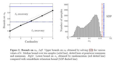
Both programs check a condition on a constant \alpha_k. The study of the value of \alpha_k with small matrices could allow one to investigate low order models as well as specific dictionaries.... These two programs are prominently listed in the measurement matrix section of the Big Picture.

In math at UAH, there will be a talk on Compressive Sampling by Brian Robinson, Center for Applied Optics, UA Huntsville, February 27, 2009, 219 Shelby Center, 3:00 (Refreshements at 2:30). The abstract of his talk is:

Conventional sampling is ruled by the Whittaker-Shannon Theorem, which states that, in order to faithfully recover a signal from a set of discrete samples, the samples must be taken with a frequency (the Nyquist frequency) which is twice the highest frequency present in the original signal. Under this regime, the sampling function is the classical comb function, consisting of a train of delta functions equally spaced with a period that is the reciprocal of twice the highest frequency in the signal. This principle underlies nearly all signal sampling protocols used in contemporary electronic devices. As it turns out, however, this method of sampling is not optimal. In other words, there are other methods that require far fewer samples than sampling with the canonical "spike" basis of W-S theory. Compressed Sensing (CS) is a novel sensing/sampling paradigm that goes against the common wisdom in data acquisition in that it demonstrates the feasibility of reconstructing data sets to a high degree of fidelity (and even exactly), with far fewer samples than is required by the W-S sampling paradigm. It is important to note that the methods are also robust to noise. CS relies on two related phenomena to make this possible: sparseness and incoherence. The properties of CS were largely discovered by applied mathematicians working in the field of probability theory and it has profound implications for practical systems such as optical imaging systems. In this talk we will illuminate the ideas of CS theory, discuss the roles of sparseness and incoherence, talk about the relationship that randomness plays in constructing a suitable set of sensing waveforms, and talk about the practical applications of this theory to modern sensing systems.

I got a request recently and the reason I am posting it is because I believe that many would be beginners have exactly the same question:

I have problems on how to calculate the coherence of CS, especially on sampling partial fouier coefficients and renconstruct the image in wavelet domain. This problem is specific for sparse MRI.

argmin ||x|| s.t. y=phi*F*psi*x

This equation is for noise-free MRI.

psi is the sparsifying transform,e.g.wavelet, F is the fourier operator, phi is the random sampling mask in MRI. Often, we acquire the raw data in MRI scanner according to phi.*mask.

For a normal MRI image with size 512*512,

My problems are:

1. Dictionary of visible basis of 2D wavelet or 2D fourier are very large, since each basis is equal to the size of image 512*512, which is 262144 as a long column, I do not think it is possible to construct the wavelet basis W and fourier basis F directly. Do you have any comments on this ? I am considering the @operator in matlab.

2. For sparse MRI, A=phi*F*psi, am I right ?

I am puzzled on the questions for a lot time and read related literatures many times.

Could you provide me some help on this? Did you collect the code for caculating the coherence for large data.

To what I responded:

You really need to look at Sparco, in particular the different set of problems solved for guidance:

http://www.cs.ubc.ca/labs/scl/sparco/index.php/Main/Problems

for every examples, there is the attendant code such as problem 503

http://www.cs.ubc.ca/labs/scl/sparco/index.php/Main/problem503.html

In any event, I think that yes, you will need the @operator to implement your wavelet basis unless there is an example in the sparco suite that does better.

From arxiv, John Langford has followed on his thoughts on error correcting codes (see his first comment when I guest blogged on his blog). The paper is Multi-Label Prediction via Compressed Sensing by Daniel Hsu, Sham Kakade, John Langford, Tong Zhang. The abstract reads:

We consider multi-label prediction problems with large output spaces under the assumption of output sparsity -- that the target vectors have small support. We develop a general theory for a variant of the popular ECOC (error correcting output code) scheme, based on ideas from compressed sensing for exploiting this sparsity. The method can be regarded as a simple reduction from multi-label regression problems to binary regression problems. It is shown that the number of subproblems need only be logarithmic in the total number of label values, making this approach radically more efficient than others. We also state and prove performance guarantees for this method, and test it empirically.

In a different direction, not specifically related to CS but hinting on ways to do a better job of calibrating a Random lens Imager here is a paper by Kyle Herrity, Raviv Raich and Alfred Hero, entitled Blind reconstruction of sparse images with unknown point spread function. The abstract reads:

We consider the image reconstruction problem when the original image is assumed to be sparse and when partial knowledge of the point spread function (PSF) is available. In particular, we are interested in recovering the magnetization density given magnetic resonance force microscopy (MRFM) data, and we present an iterative alternating minimization algorithm (AM) to solve this problem. A smoothing penalty is introduced on allowable PSFs to improve the reconstruction. Simulations demonstrate its performance in reconstructing both the image and unknown point spread function. In addition, we develop an optimization transfer approach to solving a total variation (TV) blind deconvolution algorithm presented in a paper by Chan and Wong. We compare the performance of the AM algorithm to the blind TV algorithm as well as to a TV based majorization-minimization algorithm developed by Figueiredo et al.

We don't many non-linear results but this is one: Sparse Regularization with lq Penalty Term by Markus Grasmair, Markus Haltmeier and Otmar Scherzer. The abstract reads:

We consider the stable approximation of sparse solutions to non-linear operator equations by means of Tikhonov regularization with a subquadratic penalty term. Imposing certain assumptions, which for a linear operator are equivalent to the standard range condition, we derive the usual convergence rate O(sqrt(\delta) of the regularized solutions in dependence of the noise level \delta Particular emphasis lies on the case, where the true solution is known to have a sparse representation in a given basis. In this case, if the differential of the operator satisfies a certain injectivity condition, we can show that the actual convergence rate improves up to O(\delta).

Credit photo : me and using affine matching with ASIFT ( http://mw.cmla.ens-cachan.fr/megawave/demo/asift ) to show the correspondance between two pictures translated from one another.

CS: ExCoV: Expansion-Compression Variance-component Based Sparse-signal Reconstruction, CS approach to time-frequency localization

Kun Qiu a reader of this blog, just let me know of the availability of an upcoming conference paper entitled:



ExCoV: Expansion-Compression Variance-component Based Sparse-signal Reconstruction from Noisy Measurements by Aleksandar Dogandžić and Kun Qiu. The abstract reads:

We present an expansion-compression variance component based method (ExCoV) for reconstructing sparse or compressible signals from noisy measurements. The measurements follow an underdetermined linear model, with noise covariance matrix known up to a constant. To impose sparse or compressible signal structure, we define high- and low-signal coefficients, where each high-signal coefficient is assigned its own variance, low-signal coefficients are assigned a common variance, and all the variance components are unknown. Our expansion-compression scheme approximately maximizes a generalized maximum likelihood (GML) criterion, providing an approximate GML estimate of the high-signal coefficient set and an empirical Bayesian estimate of the signal coefficients.We apply the proposed method to reconstruct signals from compressive samples, compare it with existing approaches, and demonstrate its performance via numerical simulations.

The authors have also made a webpage hosting the ExCoV implementation. It is listed in the reconstruction section of the Big Picture.

I recently talked about a seminar by Patrick Flandrin earlier but as Pierre Borgnat mentioned to me it was postponed until March 5th, 2009 at 11 am at the SCAM (Séminaire Cristolien d'Analyse Multifractale, Université de Paris 12--Val-de-Marne, salle : P3-036) . The title of the talk is: Une approche "compressed sensing" pour la localisation temps-fréquence ( or Time-frequency localization from sparsity constraints) The summary in English is:

In the case of multicomponent AM-FM signals, the idealized representation which consists of weighted trajectories on the time-frequency (TF) plane, is intrinsically sparse. Recent advances in optimal recovery from sparsity constraints thus suggest to revisit the issue of TF localization by exploiting sparsity, as adapted to the specific context of (quadratic) TF distributions. Based on classical results in TF analysis, it is argued that the relevant information is mostly concentrated in a restricted subset of Fourier coefficients of the Wigner-Ville distribution neighbouring the origin of the ambiguity plane. Using this incomplete information as the primary constraint, the desired distribution follows as the minimum $\ell_1$-norm solution in the transformed TF domain. Possibilities and limitations of the approach are demonstrated via controlled numerical experiments, its performance is assessed in various configurations and the results are compared with standard techniques. It is shown that improved representations can be obtained, though at a computational cost which is significantly increased.

The initial paper on which this presentation is based on can be found here.

CS: Open coffee talk questions, SpaRSA on the GPU, Dequantizing Compressed Sensing (ct'd)

. Round Trip Flight to Durham, NC: $ 996.57
. Two nights at the Washington Duke Inn and Golf Club: $274.23
. Attending the Compressive Sensing Workshop: $250
. Enjoying like minded folks while reading Nuit Blanche at the coffee breaks: Priceless.

While a lot of you are in the same room, here are a set of questions that might deserve some attention. Some of you may want to talk amongst yourselves on these issues.

In a recent NA-Digest, Jack Dongarra mentioned the following:

From: Jack Dongarra
Date: Mon, 9 Feb 2009 14:05:55 -0500
Subject: Linear algebra software survey request

We are planning to update the survey of freely available software for the solution of linear algebra problems. The September 2006 version of the survey can be found at: http://www.netlib.org/utk/people/JackDongarra/la-sw.html.

The aim is to put in “one place” the source code that is freely available for
solving problems in numerical linear algebra, specifically dense, sparse direct and iterative systems and sparse iterative eigenvalue problems. Please send me updates and corrections. I will post a note on the na-digest when the new list is available.
Thanks,
Jack

It turns out that in CS, linear algebra problems are being solved but it seems to me that we have not collectively connected to the older and successful LAPACK community. Maybe we should or ...maybe not. Jack responded to my request of the inclusion of a list of the current CS solvers by a "a bit too far afield" response. I agree but as in all disruptive technologies, it is just a question of time before we overtake the entire field of linear algebra :) . On the other hand should we also have a similar table such as this one on top of the mere listing given in the big picture ? and if so, what should the columns be ? (your thoughts are welcomed in the comment section that I will synthesize later).

In a different area, I was asked recently about a set of benchmark against which a solver could be confronted to. I mentioned the set of problems listed in the SPARCO suite. Should we have more of these problems in this set ? Could we get some of the hardware folks to provide different series of measurements to this set of benchmark?

With regards to the stats of this blog, every entry is seen through Google reader by 174 people and through Feedburner by about 94 people. The hit count directly to the blog amount to about 300 per day while about 66 people receive every entry directly in their mailboxes. The Compressive Sensing Study Group on Linkedin now has 105 members.

Following up on the entry on sunday, I talked to Arkadi Nemirovski, who updated his site where there are now two versions of the algorithm implemented in On verifiable sufficient conditions for sparse signal recovery via L1 minimization by Anatoli Juditsky and Arkadi Nemirovski. They are available at this site:

http://sites.google.com/site/testsensingmatrices/

It complements well the other paper entitled Testing the Nullspace Property using Semidefinite Programming by Alexandre d'Aspremont and Laurent El Ghaoui where the NSProp implementation is now available at:

http://www.princeton.edu/~aspremon/NSPcode.htm

As I said earlier, these two implementations may be game changers in that they might replace the traditional reliance on the restricted isometry property (RIP). Both programs check a condition on a constant \alpha_k. The study of the value of \alpha_k with small matrices could allow one to investigate low order models as well as specific dictionaries.... These two programs are prominently listed in the measurement matrix section of the Big Picture.

A month ago, I mentioned the release of an implementation of the SpaRSA algorithm. It looks like it can even go faster now thanks to Sangkyun Lee and Stephen Wright who implemented it on the GPU and released the implementation on this site. From that page:

Implementing Algorithms for Signal and Image Reconstruction on Graphical Processing Units, submitted, 2008.


This site contains GPU codes for compressed sensing and image denoising/deblurring:

• In compressed sensing, we implemented a simple version of the SpaRSA algorithm described by Wright, Nowak, and Figueiredo [1], using randomly chosen rows of discrete cosine transform (DCT) matrix as the sensing matrix.
• In image denoising/deblurring, we implemented the PDHG algorithm of Zhu and Chen [2], which solves the Rudin-Osher-Fatemi formulation with total variation regularization.

All GPU codes compile into Matlab mex binaries, so users can process data and pass them to our GPU routines in Matlab. Our GPU codes require CUDA-enabled GPUs from NVIDIA.

I have added this page to the Compressive Sensing Hardware page. Let us also note the SpaRSA matlab implementation is now at version 2.0.

Yesterday, I featured Dequantizing Compressed Sensing with Non-Gaussian Constraints by Laurent Jacques, David Hammond, and M. Jalal Fadili and followed up with one of those usual dumb questions to Laurent:

How does your solver compared to the one studied by Petros Boufounos and Richard Baraniuk in the 1-Bit Compressive Sensing paper ?

The short answer was:

We haven't tested yet BPDQ on this particular extreme coding.

Laurent also provided a somewhat longer answer:

But let me explain what is similar and different with Petros and Rich's method:

Let x be a signal (sparse or compressible) and let Phi be a Gaussian random sensing matrix.

In the 1-bit compressed sensing model of the paper of Petros Boufounos and Richard Baraniuk, only the sign of (Phi x) is known at the decoder. They propose then to reconstruct the signal by altering the common Basis Pursuit program in two aspects. First, they replace the fidelity term by a Quantization Consistency (QC) term, i.e. the fact that the sign of the remeasured signal candidate must provide the same measurement vector. Second, since the amplitude of the signal is lost in the sign operation, they propose to realize the BP minimization on the sphere of unit norm signals to avoid a vanishing solution. This leads however to a non-convex spherical constraint. They finally solve practically the program by first regularizing the problem on a smoothed version of the QC constraint, and second by running a projected gradient minimization to force to problem to stay on the sphere.
This method was the first attempt to really introduce the QC constraint into the Compressed Sensing formalism, while other methods relied on handling the quantization distortion on the measurements as a common noise in the Basis Pursuit DeNoise (BPDN) program. In the end, the experimental results provided by this 1-Bit CS decoder were interesting compared to the common BPDN treatment with a gain of several dBs.

Our research improves this first approach on a couple of points. First, we wanted to bring a solution for any number of bits (from 1 to many), i.e. any quantization bin width for a uniform quantization model. Second, our decoder had to be closer to the Quantization Consistency, i.e. the fact that requantizing the measurement of the reconstructed signal has to reproduce the known quantized measurement vector. Third, we desired convex constraints so that we could solve it by the versatile techniques of proximal methods and monotone operator splitting (the Douglas Rachford splitting for our case). And finally, our decoder had to be controlled by the theory, i.e. we wanted to bound the approximation error committed by the quantization noise and by possible deviation from the exactly sparse signal model, i.e. the signal compressibility, as it was already existing for the BPDN decoder.

This is why we introduced these Basis Pursuit DeQuantizer (BPDQ) of moment p for p\ge 2. In their foundations, they are adapted to signal reconstruction from measurement vector corrupted by any noise of bounded \ell_p norm since this norm replace the \ell_2 norm used in the BPDN fidelity term. Let me insist on the fact that we are not touching to the sparsity term that is still expressed in the \ell_1 norm as before. The programs BPDQ_p are really introduced to answer to one question: what is a good fidelity term adapted to a non-gaussian noise, as it is the case of the uniform quantization noise. I want to avoid any confusion with other (important but unconnected) research where the \ell_1 sparsity term is replaced by the \ell_q non-convex norm (with q \le 1).

Interestingly, if the sensing matrix satisfies a generalized Restricted Isometry Property of moment p, i.e. a RIP variant bounding the \ell_p norm (p \ge 2) of the random projection of sparse signals (a property that is also satisfied by Gaussian random matrices with high probability), the BPDQ decoders have the desired stability behaviour, i.e. the "instance optimality".

In addition, for noise due to uniform quantization of measurements, we observe an interesting effect. When we work in oversampled situation where the number m of measurements is much higher than required to have the RIP_p, the part of the BPDQ approximation error due to the quantization noise is divided by \sqrt{p+1}. Therfore, when allowed, increasing the moment p thus decreases the approximation error! This is for us really the indication that the quantization noise is handled more faithfully.

To come back to the initial comparison with the 1-bit compressed sensing of Petros Boufounos and Richard Baraniuk, their proposed method is very close to our BPDQ when p=infinity. Indeed, 1-bit quantization consists also in taking the bin width equal the sup-norm of Phi x. The fidelity term for p=infinity induces then the previous sign constraint. Notice that we do not have to work on the unit signal sphere since we add the knowledge of alpha in the coding/decoding scenario. I'm quite sure therefore that in the extreme 1-bit regime our BPDQ for p=infinity will produce results comparable to those of the initial 1-bit CS decoder. However, in oversampled situations, i.e. when m is high, the moment p can be chosen large (making the \ell_p constraint very close to the \ell_infinity one), and our decoders provides theoretically and experimentally decreasing approximation error by working closer to the Quantization Consistency.

Thank you Laurent!

Credit photo: me. That day was cold!

CS: Dequantizing Compressed Sensing with Non-Gaussian Constraints, A request for Collaboration.

Laurent Jacques just let me know of a paper and companion technical report on CS and the quantization of measurements. Here they are:

Dequantizing Compressed Sensing with Non-Gaussian Constraints by Laurent Jacques, David Hammond, and M. Jalal Fadili

In this paper, following the Compressed Sensing paradigm, we study the problem of recovering sparse or compressible signals from uniformly quantized measurements. We present a new class of convex optimization programs, or decoders, coined Basis Pursuit DeQuantizer of moment p (BPDQp), that model the quantization distortion more faithfully than the commonly used Basis Pursuit DeNoise (BPDN) program. Our decoders proceed by minimizing the sparsity of the signal to be reconstructed while enforcing a data fidelity term of bounded l_p-norm, for 2 \lt p \le \infty. We show that in oversampled situations the performance of the BPDQp decoders are significantly better than that of BPDN, with reconstruction error due to quantization divided by sqrt(p + 1). This reduction relies on a modified Restricted Isometry Property of the sensing matrix expressed in the l_p-norm (RIP_p); a property satisfied by Gaussian random matrices with high probability. We conclude with numerical experiments comparing BPDQp and BPDN for signal and image reconstruction problems.

and the attendant technical report: Dequantizing Compressed Sensing: When Oversampling and Non-Gaussian Constraints Combine by Laurent Jacques, David Hammond, and M. Jalal Fadili

After inquiring on the subject, David Hammond also let me know that:

We are planning on releasing the BPDQ solver code upon acceptance of a journal paper; so the time is unclear.

In a different direction, Brien Housand sent the following request on both this blog and the linkedin group discussion forum:

Seeking partner from Academic or non-profit research institute for multi-spectral Compressive Sensing project – paper study. Combine your knowledge of Compressive Sensing algorithms with our skills at Electro-Optical sensor design.

Contact: Brien Housand
Email: bhousand@dsci.com

After 6 months since its inception, the Compressive Sensing Study Group on LinkedIn now has 100 members.

Credit photo: me. A view of Geneva and the Mont-Blanc mountain.

CS: Testing the Nullspace Property using Semidefinite Programming and attendant NSProp code.

In a recent entry, I mentioned the utmost importance of this subject: How can one find if a given rectangular measurement or multiplexing matrix has the property of allowing recoverability of sparse signals or unknowns. Most papers are currently using the convenient Restricted Isometry Property but it is thought that this is an unnecessarily tight property. Alexandre d'Aspremont and Laurent El Ghaoui have now updated to version 3 their preprint entitled: Testing the Nullspace Property using Semidefinite Programming. Because it is important work for the whole field, I am pasting the abstract again:

Recent results in compressed sensing show that, under certain conditions, the sparsest solution to an underdetermined set of linear equations can be recovered by solving a linear program. These results rely on nullspace properties of the system matrix. So far, no tractable algorithm is known to test these conditions and most current results rely on asymptotic properties of sparse eigenvalues of random matrices. Given a matrix A, we use semidefinite relaxation techniques to test the nullspace property on A and show on some numerical examples that these relaxation bounds can prove perfect recovery of sparse solutions with relatively high cardinality.

As I had mentioned earlier, the reason for Version 3 is because (as mentioned in the arxiv page):

The J&N code in the last version did not run to full precision. This version thus includes updated (and significantly different) numerical results comparing both LP and SDP relaxations. Numerical results on the randomization lower bound were also added

What is also noteworthy and wasn't available in previous versions of the draft is the attendant code. The NSProp implementation is now available here:

http://www.princeton.edu/~aspremon/NSPcode.htm

Oustanding! Now let me point to the conclusion of the paper:

We have detailed a semidefinite relaxation for the problem of testing if a matrix satisfies the nullspace property defined in Cohen et al. (2006). This relaxation matches the linear programming relaxation in Juditsky and Nemirovski (2008) when k = 1 but is not as tight for larger values of k. On the other hand, it also produces a tractable lower bound on the objective value which does not require solving a (potentially exponentially long) sequence of convex optimization problems as in Juditsky and Nemirovski (2008). In particular, our results prove that both LP and SDP relaxations on α1 are tight for the Gaussian and Bernoulli matrices tested here. We can also remark that the matrix A only appears in the relaxation (9) in “kernel” format A^T A, where the constraints are linear in the kernel matrix A^T A. This means that this relaxation might allow sparse experiment design problems to be solved, while maintaining convexity. Of course, these small scale experiments do not really shed light on the actual performance of both relaxations on larger, more realistic problems. In particular, applications in imaging and signal processing would require solving problems where both n and k are several orders of magnitude larger than the values considered in this paper or in Juditsky and Nemirovski (2008) and the question of finding tractable relaxations or algorithms that can handle such problem sizes remains open. Also, while empirical evidence suggests that our relaxation is quite tight for certain types of random matrices (and that it matches the LP relaxation on α1, which achieves order √k for matrices satisfying the restricted isometry property at order k), we could not, at this point, produce explicit bounds on the recovery threshold of this semidefinite relaxation.

I realize that more realistic problems might be out of reach because of time constraints, but then again, I believe it is just a question of time that we either have a theoretical breakthrough in this area or we have more powerful tricks and machinery to compute this bound in a short amount of time for large rectrangular matrices. For those of you who just find out about this subject, you may to check my previous entry on this issue. On that subject, I am still looking to the re-availability of the J&N code.

CSJob: Compressed sensing theory and algorithms with particular application to dynamic MRI

Mike Davies just let me know of the following at the University of Edinburgh:

We have another job vacancy for a research fellow in compressed sensing!

Research Fellow in "Compressed sensing theory and algorithms with particular application to dynamic MRI"

It has been added to the Compressive Sensing jobs section.

CS: Compressive Light Transport Sensing

Let's take a look at a very noteworthy contribution as it clearly has impact on solving the linear transport equation (an interest of mine).

Here is a new paper entitled Compressive Light Transport Sensing ( a previous technical report can be found on this site) by Pieter Peers, Dhruv Mahajan, Bruce Lamond, Abhijeet Ghosh, Wojciech Matusik and Ravi Ramamoorthi. The abstract reads:

In this article we propose a new framework for capturing light transport data of a real scene, based on the recently developed theory of compressive sensing. Compressive sensing offers a solid mathematical framework to infer a sparse signal from a limited number of nonadaptive measurements. Besides introducing compressive sensing for fast acquisition of light transport to computer graphics, we develop several innovations that address specific challenges for image-based relighting, and which may have broader implications. We develop a novel hierarchical decoding algorithm that improves reconstruction quality by exploiting interpixel coherency relations. Additionally, we design new nonadaptive illumination patterns that minimize measurement noise and further improve reconstruction quality. We illustrate our framework by capturing detailed high-resolution reflectance fields for image-based relighting.

The teaser photo shown above has the following caption:

Three scenes captured using only 1000 non-adaptive compressive measurements, and relit using a novel conditions. The 128x128 reflectance functions of each camera pixel is reconstructed using our hierarhical reconstruction algorithm using 128 Haar wavelet coefficients per function from the observed compressive measurements.

This is outstanding.

CS: Simple Deterministically Constructible RIP Matrices with Sublinear Fourier Sampling Requirements

That is interesting! Simple Deterministically Constructible RIP Matrices with Sublinear Fourier Sampling Requirements by Mark Iwen. The abstract reads:

We present a deterministic number theoretic construction for matrices with the Restricted Isometry Property (RIP). Furthermore, we show that the number theoretic properties of our RIP matrices allow their products with Discrete Fourier Transform (DFT) matrices to be well approximated via a few highly sparse matrix multiplications. Hence, our RIP matrices may be approximately multiplied by the DFT of any input vector in sublinear-time by reading only a small fraction of its entries. As a consequence, we obtain small deterministic sample sets which are guaranteed to allow the recovery of near-optimal sparse Fourier representations for all periodic functions having an integrable second derivative over a single period. Explicit bounds are provided for the sizes of our RIP matrices, the sizes of their associated sublinear Fourier sampling sets, and the errors incurred by quickly approximating their products with DFT matrices. The Fourier sampling requirements obtained herein improve on previous deterministic Fourier sampling results in [1], [2].

CS: Rice Compressive Sensing website facelift, Change in addresses links on the Rice Site.

Mark Davenport just let me know that the Rice Compressive Sensing page has gotten a facelift and they are now using a Content Management System that allows them to boost their ability to make available the different preprints in the field. This is great. I can certainly empathize with a more systematic way to do this. A minor side effect of this migration affects the Nuit Blanche links to preprints hosted on their site. If you surf on their site, you will notice nothing,. However, if you click on a link listed here on this blog with a preprint hosted at the Rice site, then you will likely get an error. No biggie, you just need to change a little bit the address. As Mark points out:

However, the one unfortunate byproduct is that the URL for all of the papers that were actually hosted on our site has changed from

http://dsp.rice.edu/cs/papername.pdf

to

http://dsp.rice.edu/files/cs/papername.pdf

I realize this is a huge annoyance - but I just thought that I would let you know since you probably have linked to papers hosted on our site in the past, and hence those links will now go dead. I tried to keep the papers where they were, but there was just no way to get our CMS to let us both put a directory of files at the url "cs" and keep our page located at the same spot.

Thanks Mark!. I don't think the blog will be affected that much. For one, I generally link to preprints listed on the authors' pages. I also link to the other known authors so that eventually the preprints are also likely to be found on the other authors' site. This is one of the reason I keep on insisting that students (yes even undergraduates) should have their own site independent of their universities. For those of you considering this, please check the Sherpa/Romeo, Publisher copyright policies & self-archiving database to make sure of the documents you can archive on your site. To finish this note, (via this blog) and borrowing from John Baez-comment, ending a thread on the n-category cafe’s popularity starting here.

“Anyway, it’s clear we have masses of followers. Now it’s time to take over the world.”

CS:Unified Approach to Sparse Signal Processing, Using the IHT Algo, Optimal CS Algo,CfP Signal Processing, Stephen's Boyd Class on Youtube, SODA

I'll be in a place where The Google and the Interwebs have trouble reaching people. So this may look like a long post but I have not written any more post to be published later this week.

From Arxiv we have: A Unified Approach to Sparse Signal Processing by Farokh Marvasti, A. Amini, F. Haddadi, Mahdi Soltanolkotabi, Babak Khalaj, Akram Aldroubi, Sverre Holm, Saeid Sanei, Jonathon Chambers. The abstract reads:

A unified view of sparse signal processing is presented in tutorial form by bringing together various fields. For each of these fields, various algorithms and techniques, which have been developed to leverage sparsity, are described succinctly. The common benefits of significant reduction in sampling rate and processing manipulations are revealed. The key applications of sparse signal processing are sampling, coding, spectral estimation, array processing, component analysis, and multipath channel estimation. In terms of reconstruction algorithms, linkages are made with random sampling, compressed sensing and rate of innovation. The redundancy introduced by channel coding in finite/real Galois fields is then related to sampling with similar reconstruction algorithms. The methods of Prony, Pisarenko, and MUSIC are next discussed for sparse frequency domain representations. Specifically, the relations of the approach of Prony to an annihilating filter and Error Locator Polynomials in coding are emphasized; the Pisarenko and MUSIC methods are further improvements of the Prony method. Such spectral estimation methods is then related to multi-source location and DOA estimation in array processing. The notions of sparse array beamforming and sparse sensor networks are also introduced. Sparsity in unobservable source signals is also shown to facilitate source separation in SCA; the algorithms developed in this area are also widely used in compressed sensing. Finally, the multipath channel estimation problem is shown to have a sparse formulation; algorithms similar to sampling and coding are used to estimate OFDM channels.

Supporting the Sparsify recent Version 0.4, here are two papers:

How To Use The Iterated Hard Thresholding Algorithm by Thomas Blumensath and Mike Davies. The abstract reads:

Several computationally efficient algorithms have been shown to offer near optimal recovery of sparse signals from a small number of linear measurements. However, whilst many of the methods have similar guarantees whenever the measurements satisfy the so called restricted isometry property, empirical performance of the methods can vary significantly in a regime in which this condition is not satisfied. We here modify the Iterative Hard Thresholding algorithm by including an automatic step-size calculation. This makes the method independent from an arbitrary scaling of the measurement system and leads to a method that shows state of the art empirical performance. What is more, theoretical guarantees derived for the unmodified algorithm carry over to the new method with only minor changes.

A Simple, Efficient and Near Optimal Algorithm for Compressed Sensing by Thomas Blumensath and Mike Davies. The abstract reads:

When sampling signals below the Nyquist rate, efficient and accurate reconstruction is nevertheless possible, whenever the sampling system is well behaved and the signal is well approximated by a sparse vector. This statement has been formalised in the recently developed theory of compressed sensing, which developed conditions on the sampling system and proved the performance of several efficient algorithms for signal reconstruction under these conditions. In this paper, we prove that a very simple and efficient algorithm, known as Iterative Hard Thresholding, has near optimal performance guarantees rivalling those derived for other state of the art approaches.

Laurent Duval just let me know of a new Call for Papers:

Call for papers Special issue on Advances in Multirate Filter Bank Structures and Multiscale Representations
Scope
A century after the first outbreak of wavelets in Alfred Haar’s thesis in 1909, and twenty years after the advent of Multiresolution Analysis, filter banks and wavelet transforms lie at the heart of many digital signal processing and communication systems. During the last thirty years, they have been the focus of tremendous theoretical advances and practical applications in a growing digital world. They are for instance present, as local linear expansions, at the core of many existing or forthcoming audio, image or video compression algorithms. Beyond standards, many exciting developments have emerged in filter banks and wavelets from the confrontation between scientists from different fields (including signal and image processing, computer science, harmonic analysis, approximation theory, statistics, bioengineering, physics). At their confluence, multiscale representations of data, associated with their efficient processing in a multirate manner, have unveiled tools or refreshed methods impacting the whole data management process, from acquisition to interpretation, through communications, recovery and visualization. Multirate structures naturally shelter key concepts such as the duality between redundancy and sparsity, as well as means for extracting low dimensional structures from higher ones. In image processing in particular, various extensions of wavelets provide smart linear tools for building insightful geometrical representations of natural images. The purpose of this special issue is to report on recent progresses performed and emerging trends in the domain of multirate filter banks and multiscale representations of signals and images. Answers to the challenge of handling an increasing demand of information extraction and processing from large data sets will be explored.
Topics (not exclusive)

• Sampling theory, compressive sensing
  
• Sparse representations
  
• Multiscale models
• Multiscale processing: interpolation, inpainting, restoration,
• Wavelet shrinkage and denoising
• Oversampled filter banks, discrete frames
• Rational and non-uniform multirate systems
• Directional, steerable filter banks and wavelets
• Nonlinear filter banks
• (Multidimensional) filter bank design and optimization
• Hybrid analog/digital filter banks
• Fast and low-power schemes (lifting, integer design)
• Multiscale and multirate applications to source and channel coding, equalization, adaptive filtering, ....

Important dates:

• Deadline for submission: 15 December 2009
  
• First round of reviews/decisions: 1 April 2010
  
• Resubmission of revised papers: 1 July 2010
  

Submission
Guidelines for authors can be found at http://www.elsevier.com/locate/sigpro. Authors should submit their manuscripts before the submission deadline via http://ees.elsevier.com/sigpro/ selecting ‘‘Special Issue: Multirate/Multiscale’’ as Article Type.

I already knew of the Stephen Boyd's class on Youtube such as this one:

What I did not realize was that somebody had gone through the pain of transcribing these videos. Wow, just Wow. For instance the text of the video above is found here. The rest of Stephen Boyd's excellent class can be found here and here with the attendant text.

The Papers presented at SODA are now available. Among the ones, I am surely going to be reading (after some advice from Frank Nielsen that I should know about Coresets)

• The Johnson-Lindenstrauss lemma almost characterizes Hilbert space, but not quite by William B. Johnson and Assaf Naor.
• Constructing Laplace Operator from Point Clouds in Rd by Mikhail Belkin, Jian Sun, Yusu Wang.
• Coresets and Approximate Clustering for Bregman Divergences by Marcel R. Ackermann and Johannes Blomer.
• Overcoming the l_1 Non-Embeddability Barrier:Algorithms for Product Metrics by Alexandr Andoni, Piotr Indyk, Robert Krauthgamer.

Over at the CAVE lab at Columbia, they just released the title of an intriguing technical report entitled "Generalized Assorted Pixel Camera: Post-Capture Control of Resolution, Dynamic Range and Spectrum," by F. Yasuma, T. Mitsunaga, D. Iso, and S.K. Nayar. Yet the pdf link does not seem to work for the moment.

Also of interest is theASPLOS 2008 Tutorial : CUDA: A Heterogeneous Parallel Programming Model for Manycore Computing blog entry.

In a different area, Shenzou VII passed by the International Space Station, here is a simulation by the folks at AGI. In a different area, I look forward to seeing how the recent collision between an Iridium satellite and a Russian satellite will disturb that low earth orbit environment with space debris. To see how bad this collision is, you need to check out the calculations on the Bad Astronomy blog. Have you ever been rearsided by something at 17,000 mph ? Let us recall that we are really close to a prompt critical situation in this area and this is worrisome as most of our daily lives depends on Satellites these days.

CS: Sparse Approximation and Atomic Decomposition, SPARS'09 program, Counter Braids, trending in the stock market, L_0 reconstruction

Bob Sturm, a reader of this blog, just released his recently defended Ph.D. thesis entitled Sparse Approximation and Atomic Decomposition: Considering Atom Interactions in Evaluating and Building Signal Representations. The attendant slides of that defense can be found here. The abstract of the thesis reads:

This dissertation makes contributions to the sparse approximation and efficient representation of complex signals, e.g., acoustic signals, using greedy iterative descent pursuits and overcomplete dictionaries. As others have noted before, peculiar problems arise when a signal model is mismatched to the signal content, and a pursuit makes bad selections from the dictionary. These result in models that contain several atoms having no physical significance to the signal, and instead exist to correct the representation through destructive interference. These ``spurious'' terms greatly diminish the efficiency of the generated signal model, and hinder the useful application of sparse approximation to signal analysis (e.g., source identification), visualization (e.g., source selection), and modification (e.g., source extraction). While past works have addressed these problems by reformulating a pursuit to avoid them, such as adding restrictions to the content of a dictionary, in this dissertation we use these corrective terms to learn about the signal, the pursuit algorithm, the dictionary, and the created model. Our thesis is essentially that a better signal model results when a pursuit builds it considering the interaction between the atoms. We formally study these effects and propose novel measures of them to quantify the interaction between atoms in a model, and to illuminate the role of each atom in representing a signal. We then propose and study three different ways of incorporating these new measures into the atom selection criteria of greedy iterative descent pursuits, and show analytically and empirically that these interference-adaptive pursuits can produce models with increased efficiency and meaningfulness, e.g., the direct correspondence between an atom and specific signal content. Finally, we propose creating a higher-level model of the decomposed signal by agglomerating the atoms of a representation into molecules based on a set of similarity criteria, and compare this method with a previous pursuit that builds molecules simultaneously with the decomposition process. In both cases, we find that the resulting molecules have a more clear relationship with the signal content.

One can note that he is going to have to continue his postdoc in Paris. Life ain't fair :-)

The SPARS'09 conference has just released the list of the talks that will be featured there. It is here. It looks like a very interesting and worthy program.

Laurent Gosse, a trader it seems, writes about the trend of the CAC-40, the french local stock index using what he calls Compressed Sensing. I am not quite sure but it looks like detrending using l1 regularization.

There is also a new version of the presentation entitled Toward 0-norm Reconstruction, and a Nullspace Technique for Compressive Sampling by Christine Law and Gary Glover.

Finally, Yi Lu  and Balaji Prabhakar continue investigating their counter braid work with  Robust Counting via Counter Braids: An Error-Resilient Network Measurement Architecture. The abstract reads:

A novel counter architecture, called Counter Braids, has recently been proposed for accurate per-flow measurement on high-speed links. Inspired by sparse random graph codes, Counter Braids solves two central problems of per-flow measurement: one-to-one flow-to-counter association and large amount of unused counter space. It eliminates the one-to-one association by randomly hashing a flow label to multiple counters and minimizes counter space by incrementally compressing counts as they accumulate. The random hash values are reproduced offline from a list of flow labels, with which flow sizes are decoded using a fast message passing algorithm. The decoding of Counter Braids introduces the problem of collecting flow labels active in a measurement epoch. An exact solution to this problem is expensive. This paper complements the previous proposal with an approximate flow label collection scheme and a novel error-resilient decoder that decodes despite missing flow labels. The approximate flow label collection detects new flows with variable-length signature counting Bloom filters in SRAM, and stores flow labels in high-density DRAM. It provides a good trade-off between space and accuracy: more than 99 percent of the flows are captured with very little SRAM space. The decoding challenge posed by missing flow labels calls for a new algorithm as the original message passing decoder becomes error-prone. In terms of sparse random graph codes, the problem is equivalent to decoding with graph deficiency, a scenario beyond coding theory. The error-resilient decoder employs a new message passing algorithm that recovers most flow sizes exactly despite graph deficiency. Together, our solution achieves a 10-fold reduction in SRAM space compared to hash-table based implementations, as demonstrated with Internet trace evaluations.

Credit & Copyright: Eric J. Zbinden, Space Station in the Moon (via astronomy picture of the day)

CS: Efficient and Guaranteed Rank Minimization by Atomic Decomposition, Sparse time-frequency distributions of chirps from CS, un sujet de these.

The Rice Compressive Sensing Resource page has changed its presentation. Check it out. I think they also have gone through the pain of updating where preprints have been eventually published. Kudos to them!

We also have two papers and an annoucement for a thesis (in french).

Efficient and Guaranteed Rank Minimization by Atomic Decomposition by Kiryung Lee and Yoram Bresler. The abstract reads:

Recht, Fazel, and Parrilo provided an analogy between rank minimization and ℓ0-norm minimization. Subject to a generalized restricted isometry property, nuclear norm minimization is a guaranteed heuristic for rank minimization. The resulting semidefinite formulation is a convex problem but in practice the algorithms for it do not scale well to large instances. Instead, we explore missing terms in the analogy and propose a new heuristic which is computationally efficient and also has a performance guarantee. The heuristic is based on the atomic decomposition of the matrix variable and extends the idea in the CoSaMP algorithm for ℓ0-norm minimization. The correlation maximization rule for CoSaMP is generalized to derive a new selection rule. Combined with the recent fast low rank approximation of matrices based on randomization, the proposed algorithm can efficiently handle large scale rank minimization problems.

Sparse time-frequency distributions of chirps from a compressed sensing perspective by Patrick Flandrin, Pierre Borgnat. The abstract reads:

Considering that multicomponent chirp signals are sparse in the time-frequency domain, it is possible to attach to them highly localized distributions thanks to a compressed sensing approach based on very few measurements in the ambiguity plane. The principle of the technique is described, with emphasis on the choice of the measurement subset for which an optimality criterion is proposed.

And this one annoucement for a thesis in French, let us note hte use of sensor development for UAVs.

 

Proposition de sujet de these a l'Office National d’Études et de Recherches Aérospatiales a Chatillon. Sujet: Conception conjointe optique/traitement pour imageurs compacts

Laboratoire d’accueil à l’ONERA :

Branche : TIS

Département : DTIM

Unité : EVS

Lieu (centre ONERA) : Châtillon

Responsable ONERA : Frédéric Champagnat (EVS)

Directeur de thèse universitaire envisagé:

RÉSUMÉ :

Les dernières années ont vu se développer de nouveaux concepts de capteurs optroniques [1] qui remettent en cause les compromis de prise d’image classiques (par exemple, temps de pause/ouverture [2]), en couplant une optique non standard (par exemple, une optique multi-voies de type oeil à facettes ou une optique de type axicon diffractif) à un traitement dédié, effectué le cas échéant au vol. Corrélativement, une intense réflexion est en cours dans la communauté du traitement de signal et de l’image sur des modes d’acquisition assurant une compacité optimale du signal délivré par le capteur, activité identifiée sous l’appellation « compressed sensing » [3]. Ces évolutions sont à l’origine du projet de recherche fédérateur ONERA SPIDER, portant sur la conception de composants de perception (capteur + traitement) embarquables par exemple sur des petits drones, pour l’interprétation dynamique d’événements et de situations en milieu urbain.

Le développement de tels composants remet en cause les cloisonnements classiques entre opticiens d'une part et traiteurs d'image d'autre part, et appelle à l'optimisation conjointe capteur+traitement. Cette thèse s'inscrit dans le projet SPIDER et se déroulera dans une équipe de traitement d’image du Département de Traitement de L’information et de Modélisation (DTIM) en collaboration avec une équipe d’opticiens du Département d’Optique Théorique et Appliquée (DOTA).

L’objectif de la thèse est de contribuer à l’étude de plusieurs de ces concepts et de leur apport éventuel pour les fonctionnalités nécessaires à un système autonome comme un petit drone d’observation (reconnaissance d’objets, interprétation de scène, ego-localisation, évitement d’obstacles). A moyen terme, les concepts les plus prometteurs seront retenus pour la réalisation d’un protoype capteur+traitement et sa démonstration....

Image Credit: NASA/JPL/Space Science Institute, photo of Titan taken three days ago by Cassini.

CS: a job, Golden Ratio Radial Imaging, Model-based CS MRI, Rate Distortion Behavior of Sparse Sources, MP Shrinkage in Hilbert Spaces

Mike Davies just let me know of a job announcement for a research Fellow at the University of Edinburgh,UK for three years starting March 1, 2009. I am adding it to Compressive Sensing jobs section. Looks like The Google has not indexed it yet, woohoo ... we are going faster than The Google.

The sampling approach of the first paper/poster strangely ressembles the result by Yves Meyer, Basarab Matei featured in A variant on the compressed sensing of Emmanuel Candes (I talked about it here, here and here in reference to MRI). The paper is entitled: Highly Undersampled 3D Golden Ratio Radial Imaging with Iterative Reconstruction by Mariya Doneva, Holger Eggers , J. Rahmer , Peter Börnert and Alfred Mertins. The introduction reads:

Compressed Sensing (CS) [1,2] suggests that using nonlinear reconstruction algorithms based on convex optimization an accurate signal reconstruction can be obtained from a number of samples much lower than required by the Nyquist limit. Recently, CS was demonstrated for MR imaging from undersampled data [3, 4]. Prerequisites for a good image reconstruction are the image compressibility and the incoherence of the sampling scheme. To exploit the full potential of CS, measurement samples should be acquired at random. However, random sampling of the k-space is generally impractical. Variable density sampling schemes (radial, spiral) lead to incoherent aliasing and are also advantageous because of their higher sampling density about the k-space origin, where most of the signal energy is contained. 3D variable density sampling is potentially appropriate for CS, because the noise-like aliasing is distributed within the complete volume, allowing high undersampling factors. Image reconstruction from a low number of measurements could be very useful for dynamic 3D imaging, to reduce the often long acquisition times and thus improve temporal resolution in 3D MRI. In this work, we demonstrate the applicability of CS for 3D dynamic imaging using highly undersampled 3D radial acquisition with golden ratio profile ordering [5,6].

and from the same group of folks we also have: Model-based Compressed Sensing reconstruction for MR parameter mapping by Mariya Doneva, Christian Stehning, Peter Börnert, Holger Eggers and Alfred Mertins. The introduction reads:

Compressed Sensing [1-4] suggests that compressible signals can be reconstructed from far less samples than required by the Nyquist-Shannon sampling theorem. Signal recovery is achieved by Basis Pursuit (BP) [2] or greedy algorithms like Orthogonal Matching Pursuit (OMP) [4]. The latter has weaker performance guarantees, but it is often faster and is thus an attractive alternative to BP. Most commonly, orthonormal bases are applied as a sparsifyingtransform. However, allowing the signal to be sparse with respect to an overcomplete dictionary adds a lot of flexibility with regard to the choice of the transform and could improve the transform sparsity. MR parameter mapping measurements of relaxation times T1 and T2, diffusion coefficients, etc. require the acquisition of multiple images of the same anatomy at varying parameters, which is associated with long acquisition times. These data are described by a model with only few parameters, which could be used to design a model-based overcomplete dictionary for CS reconstruction. In this work we demonstrate this approach for the acceleration of T1 mapping data acquisition.

I also found: Rate Distortion Behavior of Sparse Sources by Claudio Weidmann, Martin Vetterli. The abstract reads:

The rate distortion behavior of sparse memoryless sources is studied. Such sources serve as models for sparse representations and can be used for the performance analysis of "sparsifying" transforms like the wavelet transform, as well as nonlinear approximation schemes. Under the Hamming distortion criterion, R(D) is shown to be almost linear for sources emitting sparse binary vectors. For continuous random variables, the geometric mean is proposed as a sparsity measure and shown to lead to upper and lower bounds on the entropy, thereby characterizing asymptotic R(D) behavior. Three models are analyzed more closely under the mean squared error distortion measure: continuous spikes in random discrete locations, power laws matching the approximately scale-invariant decay of wavelet coefficients, and Gaussian mixtures. The latter are versatile models for sparse data, which in particular allow to bound the suitably defined coding gain of a scalar mixture compared to that of a corresponding unmixed transform coding system. Such a comparison is interesting for transforms with known coefficient decay, but unknown coefficient ordering, e.g. when the positions of highest-variance coefficients are unknown. The use of these models and results in distributed coding and compressed sensing scenarios is also discussed.

Martin Vetterli also made a video presentation at ECTV'08. It is entitled Sparse Sampling: Variations on a Theme by Shannon. Other videos of the conference can be found here.

Finally, Matching Pursuit Shrinkage in Hilbert Spaces by Tieyong Zeng, and Francois Malgouyes. The abstract reads:

This paper contains the research on a hybrid algorithm combining the Matching Pursuit (MP) and the wavelet shrinkage. In this algorithm, we propose to shrink the scalar product of the element which best correlates with the residue before modifying. The study concerns a broad family of shrinkage functions. Using weak properties of these shrinkage functions, we show that the algorithm converges towards the orthogonal projection of the data on the linear space generated by the dictionary, modulo a precision characterized by the shrinkage function. In the deterministic settings, under a mild assumption on the shrinkage function (for instance, the hard shrinkage satisfies this assumption), this algorithm converges in a finite time which can be estimated from the properties of the shrinkage function. Experimental results show that in the presence of noise, the new algorithm does not only outperform the regular MP, but also behaves better than some other classical Greedy methods and Basis Pursuit Denoising model when used for detection.

Image Credit: NASA/JPL/Space Science Institute. Dione as seen by Cassini last friday.

CS: A review, Efficient Encoding of Audio Signals, Greedy Algorithms Comparison, Randomized algo, l1 solvers, Quality is Number 1 again!

Weren't Friday's papers interesting or what ? Today we have a batch of six. 

From Sparse Solutions of Systems of Equations to Sparse Modeling of Signals and Images by Alfred Bruckstein, David Donoho, Michael Elad. The abstract.

A full-rank matrix A element of R^(n×m) with n less than m generates an underdetermined system of linear equations Ax = b having infinitely many solutions. Suppose we seek the sparsest solution, i.e., the one with the fewest nonzero entries. Can it ever be unique? If so, when? As optimization of sparsity is combinatorial in nature, are there efficient methods for finding the sparsest solution? These questions have been answered positively and constructively in recent years, exposing a wide variety of surprising phenomena, in particular the existence of easily verifiable conditions under which optimally sparse solutions can be found by concrete, effective computational methods. Such theoretical results inspire a bold perspective on some important practical problems in signal and image processing. Several well-known signal and image processing problems can be cast as demanding solutions of undetermined systems of equations. Such problems have previously seemed, to many, intractable, but there is considerable evidence that these problems often have sparse solutions. Hence, advances in finding sparse solutions to underdetermined systems have energized research on such signal and image processing problems—to striking effect. In this paper we review the theoretical results on sparse solutions of linear systems, empirical results on sparse modeling of signals and images, and recent applications in inverse problems and compression in image processing. This work lies at the intersection of signal processing and applied mathematics, and arose initially from the wavelets and harmonic analysis research communities. The aim of this paper is to introduce a few key notions and applications connected to sparsity, targeting newcomers interested in either the mathematical aspects of this area or its applications.

Efficient Encoding of a Sinusoidally-Modelled Audio Signal Using Compressed Sensing by Anthony Griffin, Christos Tzagkarakis, Toni Hirvonen, Athanasios Mouchtaris and Panagiotis Tsakalidesthe abstract reads:

In this paper, the compressed sensing (CS) methodology is applied to the harmonic part of sinusoidally- modelled audio signals. As this part of the model is sparse by definition in the frequency domain, we investigate whether CS can be used for encoding this signal at low bitrates, instead of encoding the sinusoidal parameters (amplitude, frequency, phase) as current state-of-the-art methods do. CS samples signals at a much lower rate than the Nyquist rate if they are sparse in some basis, thus it is a natural choice in this context. This also has the potential benefit of moving the computational burden from the encoder to the decoder. Previous work presented an initial investigation into the performance of this scheme, and this paper demonstrates how the performance can be further improved to rival that of a state-of-the-art encoder.

A Comparative Study of Some Greedy Pursuit Algorithms for Sparse Approximation by Gagan Rath and Arabinda Sahoo. The abstract reads:

Solving an under-determined system of equations for the sparsest solution has attracted considerable attention in recent years. Among the two well known approaches, the greedy algorithms like matching pursuits (MP) are simpler to implement and can produce satisfactory results under certain conditions. In this paper, we compare several greedy algorithms in terms of the sparsity of the solution vector and the approximation accuracy. We present two new greedy algorithms based on the recently proposed complementary matching pursuit (CMP) and the sensing dictionary framework, and compare them with the classical MP, CMP, and the sensing dictionary approach. It is shown that in the noise-free case, the complementary matching pursuit algorithm performs the best among these algorithms.

In a fascinating area I briefly mentioned a year ago, here is Randomized Kaczmarz Solver for Noisy Linear Systems by Deanna Needell. The abstract reads:

The Kaczmarz method is an iterative algorithm for solving systems of linear equations Ax = b. Theoretical convergence rates for this algorithm were largely unknown until recently when work was done on a randomized version of the algorithm. It was proved that for overdetermined systems, the randomized Kaczmarz method converges with expected exponential rate, independent of the number of equations in the system. Here we analyze the case where the system Ax = b is corrupted by noise, so we consider the system Ax ≈ b + r where r is an arbitrary error vector. We prove that in this noisy version, the randomized method reaches an error threshold dependent on the matrix A with the same rate as in the error-free case. We provide examples showing our results are sharp in the general context.

Olivier Grisel pointed out the following two papers while on Twitter. they are relevant to new schemes devised for solving l1 and related reconstructions. Now the question is whether they are any faster than the current ones we already have:

An interior-point stochastic approximation method and an L1-regularized delta rule by Peter Carbonetto, Mark Schmidt and Nando de Freitas. The abstract reads:

The stochastic approximation method is behind the solution to many important, actively-studied problems in machine learning. Despite its far-reaching application, there is almost no work on applying stochastic approximation to learning problems with general constraints. The reason for this, we hypothesize, is that no robust, widely-applicable stochastic approximation method exists for handling such problems. We propose that interior-point methods are a natural solution. We establish the stability of a stochastic interior-point approximation method both analytically and empirically, and demonstrate its utility by deriving an on-line learning algorithm that also performs feature selection via L1 regularization.

and Online and Batch Learning using Forward Looking Subgradients by John Duchi, Yoram Singer. The abstract reads:

We describe, analyze, and experiment with a new framework for empirical loss minimization with regularization. Our algorithmic framework alternates between two phases. On each iteration we first perform an unconstrained gradient descent step. We then cast and solve an instantaneous optimization problem that trades off minimization of a regularization term while keeping close proximity to the result of the first phase. This view yields a simple yet effective algorithm that can be used for batch penalized risk minimization and online learning. Furthermore, the two phase approach enables sparse solutions when used in conjunction with regularization functions that promote sparsity, such as ℓ1. We derive concrete and very simple algorithms for minimization of loss functions with ℓ1, ℓ2, ℓ2^2, and ℓ1 regularization. We also show how to construct efficient algorithms for mixed-norm ℓ1/ℓq regularization. We further extend the algorithms and efficient implementations for very high-dimensional data with sparsity. We demonstrate the potential of the proposed framework in a series of experiments with synthetic datasets.

Credit photo 1: NASAWatch, the Satellite in this photo is the NOAA-N Prime satellite. I talked about the incident here. Five years later, the satellite was launched on Friday and is currently in orbit. Woohoo.

Credit photo 2: NASA/Carleton Bailie, ULA