Nuit Blanche: CS: Multiplicative Noise Effect on the Donoho-Tanner Phase Transition (Part 2)

Thursday, March 24, 2011

CS: Multiplicative Noise Effect on the Donoho-Tanner Phase Transition (Part 2)

For some reasons I cannot find the list of papers and genesis that got me thinking about this project, I thought I had already listed some amount of it in the blog. Oh well. Here we go. One of the starting point of this thought process is [1][2] but while Matthew Herman and Thomas Strohmer did a great job, I was lacking a better illustration as I am a very visual person. Their figure is a good start (below), but it would seem to me that any practicing engineer would want to have a better bird's eye view of the situation.

Because as you watch this figure and you get to think, this noise cannot be that bad. But then you read the work of Sylvain Durand, Jalal Fadili, Mila Nikolova [4] and you get hit by a wall of bricks. it's official:

It's bad. Notwithstanding a reconstruction technique devoted to removing that type of noise, it can't. Worse, the results look like an F or an R.

So the next step is to get a graphic that seems intuitive. For different reasons including some type of universality (as Remi Gribonval pointed out recently), I believe the Donoho-Tanner phase transition for sparse recovery (web page: Phase Transitions of the Regular Polytopes and Cone at University of Edinburgh.) provides such a comprehensive view.

However reading the Donoho-Tanner phase transition diagram is always difficult for me because of the hyperboles.

So from now on, unless I am mentioning otherwise, I'll draw this phase transition but with with either k/N or k on the y-axis as opposed to the traditional k/m. If you recall the convention (for us CS people):

k stands for the sparsity of the solution
m for the number of measurements or the number of equations
N for the dimension of the underlying space or the number of unknowns.
k/m is the under-sampling ratio
m/N is the over-sampling ratio

You may note that in the last figure, the x-axis or m/N goes beyond m/N = 1. In other words, we just don't look at underdetermined systems but we also look at overdetermined ones as well.

So let us look at this diagram with the least square solver (\ in Matlab). We use a perturbation \epsilon*E with E a random gaussian.

What does the graph says: here we use epsilon = 0, i.e. no noise. If the system is underdetermined (x less than 1) then the least square solver cannot find any solution to the linear system at hand. When the system is overdetermined (x greater than 1) then the solver can find a solution all the time. This solution also happen to be full (the transition cannot be easily seen but it is at y =1). So far, so good all this was expected. Now let us look at epsilon = 0.003

Now the transition has shifted a little bit to the right and it begins to have a slope. Now let us look at epsilon = 0.005, the trend continues:

Now with epsilon = 0.01, we have:

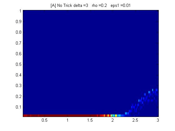
or by increasing the x-axis, we have:

This is a surprise (to me). This graph tells me that for a solution with k/N above 0.3, the least square solver cannot find that solution under 1% multiplicative noise with a linear system three times overdetermined. I think everybody kind of expects the rule of thumb that you just need additional equations to get a solution, but this is not what we see. More tomorrow....