Why L1 ?

I have had this question asked to me recently and I think the cleanest explanation from the standpoint of statistics and maximum entropy consideration lies in this entry on Bayesian inference of the median.

Looking back at some examples, when Andrew Ng [1] tries to build depth maps from monocular vision this is what he says when trying to fit test data from natural scene to statistical models:

We now present a second model that uses Laplacians instead of Gaussians to model the posterior distribution of the depths. Our motivation for doing so is three-fold. First, a histogram of the relative depths (di - dj ) empirically appears Laplacian, which strongly suggests that it is better modeled as one. Second, the Laplacian distribution has heavier tails, and is therefore more robust to outliers in the image features and error in the trainingset depthmaps (collected with a laser scanner; see Section 5.1). Third, the Gaussian model was generally unable to give depthmaps with sharp edges; in contrast, Laplacians tend to model sharp transitions/outliers better.

Obtaining a sparse (i.e. the smallest model) and a robust solution (to outliers) is the reason why he uses L1. Using L1 is also why Lawrence Carin, Shihao Ji and Ya Xue [2] use Laplace distributions in order to obtain a sparse solution in their Bayesian compressive sensing approach. The chapter in Inder Jeet Taneja's book is a nice reference to differential entropy and associated probability distributions that maximize it (in other words, given a certain type of information/assumptions on the problem what is the type of distribution that allows one to build a model with that knowledge and not more). In imaging, decomposing a scene with a dictionary of overcomplete bases using the compressed sensing approach has shown L0 to be well approximated by L1. So in effect, when one solves approximation problems with L1, many times, one is solving for L0, i.e. for the sparser solution out of the whole potentially overcomplete dictionary.

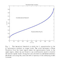
I say many times, because it also happens that combinatorial search schemes (L0) are unavoidable as shown in this paper by David Donoho and Victoria Stodden (Breakdown Point of Model When the Number of Variables Exceeds the Observations )

The "phase diagram" shown on the side marks the boundary between areas where L1 is like L0 and when L1 cannot converge to an L0 solution. [p is the number of variables. n is the number of observations and k is measure of sparsity of the underlying model] The x-axis is the level of underdeterminedness (close to 0 means very few observations compared to the number of variables) , and the y-axis is the level of sparsity of the underlying model (close to 0 means a very dense signal, close to 1 means a very sparse signal)

[1] Depth Estimation Using Monocular and Stereo Cues / 2197, Ashutosh Saxena, Jamie Schulte, Andrew Y.Ng and Learning Depth from Single Monocular Images, Ashutosh Saxena, Sung Chung, and Andrew Y. Ng. In NIPS 18, 2006. [ pdf]

[2] Bayesian compressive sensing by Shihao Ji, Ya Xue, and Lawrence Carin

[3] John Langford, Loss Function Semantics.